Name: Leo (Sunpeng) Li
Stu #: 999093421
Modified: Aug 15, 2015
The ray tracer used in the teaching of the CSCD18 course uses a naive ray-object intersection method that searches through all objects within the scene to identify the nearest hit. This is sub-optimal, as even objects that are - for example - behind the rays origin, are considered. Given the ray’s origin and direction, in addition to the locations of all the objects (in our case, triangles) within the scene, we need to find a method such that only the triangles that matter to our ray are searched, while obvious misses are ignored.
One possible solution is to employ spacial subdivision: divide the 3D scene into large chunks called bounded volumes, each containing a portion of the triangles within the scene. That way, an intersection search will be the like following:
Bounded volumes can have shapes ranging from prisms, to spheres. For simplicity however, a rectangular prism or a cube is most frequently used.
For this project, a specific form of spacial subdivision method using a octree structure is used. Casting a ray into an octree involves identifying the leaves it will hit, then processing the triangles in each of the leaves. Since the number of triangles contained within each leaf has a logarithmic relationship with the total number of triangles within the scene, we expect an exponential speed up as total triangle count increases. Indeed, this is the case as shown in performance tests.
In this report, we will go through the idea of the octree, and why it is used. The procedure for generating and ray-casting within an octree will be explained, and performance data will be presented. The results presents a significant speedup when ray-tracing scenes with large triangle counts in comparison with the naive method.
An octree is a recursive tree-like structure where each node branches into 8 children, and each child is also a node that can have their own 8 children, and so forth. The leaves of the octree are nodes that do not have any children.
For ray-tracing purposes, each node in the octree represents a cube in 3D space. They can be subdivided by slicing across each of the x, y, and z mid-planes, forming 8 identical child cubes that nests perfectly within the parent cube. This process can be repeated until a certain termination criterion is met. This termination criterion is very important, as it will determine whether or not the generated octree will be optimal for ray-casting.
Note: In this report, the term ray-tracing refers to the rendering technique, while ray-casting refers to executing ray-triangle tests within an octree spacial structure.
The simplest way to define an octree is to first assume that it is axis aligned, i.e. all the faces of the cube have one of the axis as its normal vector. Its definition then simplifies down to

When subdividing a node, its children’s size and center is calculated using the parent’s size and center. Since we are subdividing at the parent node’s mid-planes, its children will have exactly half its size. Their centers would be translated from the parent’s center by mirrored variations of the vector [size/4, size/4, size/4] depending on their location.
Indeed, there are other methods to create spacial subdivision for optimizing ray-tracing, such as Bounded Volume Hierarchies (BVH). Although BVH has been experimentally shown to be faster, We will use octrees for its simple concept, and code readability from its recursiveness.
Advantages of (but not limited to) octrees are:
A simple way to construct an octree is to completly subdivide it to a predetermined depth, giving us a leaf count of $8^{depth}$. We then do a bottom up traversal, "pruning" away any node that have expensive leaves (leaves that contain no triangles, for example). Pruning a node, as defined for an octree, is deleting its children, and all of its children's children, recursively. Based upon this idea, there are two things we need to know:
These two point are answered in the paper Octrees with near optimal cost for ray-shooting, which aims to prove that the given answers are indeed, optimal. Without going into detail about the proofs, the paper says that
To determine if we should prune a node, we run the cost function on the said node twice. Once assuming its a leaf (pruned), and another with its children intact. We compare the two costs, and keep the least expensive version of the two.
For a ray-tracer, the expensiveness of a rendering operation scales with the number of rays being traced. This is intuitive, as more rays means more intersection tests.This gives us a basis for the method of cost calculation we should use for octrees.
Since this cost function should be applicable to any scenes, we have to assume that the rays can originate from any point within the scene. This makes the surface area of the node a good value to use, as it approximates the volume of rays that will hit it. Taking into consideration the triangles within the scene, and the time it takes to find the next node within our ray traversal, we can construct the following cost function:
$$C_S(T) = \sum_{l \in L(T)} (r + |S_l|)*\lambda_{d-1}(l)$$
Where:
We can split this cost function for a node $T$ into its tree cost and object cost component:
$$\begin{align*} C_S(T) &= \sum_{l \in L(T)} (r + |S_l|)*\lambda_{d-1}(l) \\ &= \sum_{l \in L(T)} r * \lambda_{d-1}(l) + \sum_{l \in L(T)} |S_l| * \lambda_{d-1}(l) \end{align*}$$
The first summation represents the $C_t(T)$ tree cost, while the second summation representes the $C_o(T)$ object cost. We can see why they are named like so, as the tree cost estimates the cost of traversing through the given octree, while the object cost estimates the cost of finding intersections.
Note that the research paper presents $C_t(T)$ and $C_o(T)$ differently, but it's just a reformulation of what we stated above:
$$\begin{align*} C_t(T) &= \sum_{l \in L(T)} r * \lambda_{d-1}(l) \\ &= r * \sum_{l \in L(T)} \lambda_{d-1}(l) \\ &= r * \lambda_{d-1}(L(T)) \end{align*}$$
Where $\lambda_{d-1}(l)$ is expanded to sets of $L(T)$ leaves using summation, and
$$\begin{align*} C_o(T) &= \sum_{l \in L(T)} |S_l| * \lambda_{d-1}(l) \\ &= \sum_{s \in S} \lambda_{d-1}(L_s(T)) \end{align*}$$
Where $s \in S$ is an object within the scene, and $L_s(T)$ is the set of leaves intersecting with object $s$.
With the cost function, we can make a clear decision on whether or not to prune the node, or keep it as is. We execute this for all nodes while doing a bottom up traversal of $T^{complete}_{p_{max}}$, which is an octree that is fully subdivided $p_{max}$ times, containing $8^{p_{max}}$ leaf nodes.
However, there is a problem with this method, as creating $T^{complete}_{p_{max}}$ uses a large amount of memory. Even for a value as low as $p_{max}=10$, we will have $8^{10}$ leaves. Note that $p_{max}=10 \implies n = 2^{10}$, where $n$ is triangle count, since the max depth is calculated using $log_2(n)$. This is undesirable, as triangle counts for 3D scenes can get quite large.
The paper proposes the 3-greedy construction algorithm to construct octrees. It consists of a grow and prune phase. The grow phase fully subdivides a specified node $T$ 3 times (hence 3-greedy) to get $T^{complete}_3$. The prune phase executes the pruning procedure on $T^{complete}_3$ to get $T^{pruned}_3$. The process repeats for $L(T^{pruned}_3)$ until all leaves are marked as pruned, or the max depth $p_{max}$ has been reached.
Calculating $C_o(T)$ requires that we know the number of triangles contained within $L(T)$. Therefore, we need to be able to identify if a triangle $s$ is intersecting with an axis aligned bounding box (AABB) represented by the octree leaf $l$.
The method explained here is taken from Fast 3D Triangle-Box Overlap Testing by Tomas Akenine-Moller. The paper shows the equations for the overlap tests being used, but this report aims to explain how they are derived. The code can be found here.
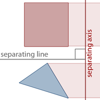
To determine if a triangle is intersecting a leaf $l$, we use the Separating Axis Theorem (SAT). In its simple form, it states that:
Two convex objects do not overlap if there exists a line (called [the separating] axis) onto which the two objects' projections do not overlap
- Wikipedia on "separating axis theorem"
The wiki page also formally proves the theorem, more generally named as "Hyperplane separation theorem" for n-dimensional Euclidean space. But for the practical case of triangle-AABB intersections, the simple definition will suffice. Also note the technical terms presented. Separating axis is the axis onto which the two convex objects are projected. The separating line is the line perpendicular to the separating axis that can be drawn between the two convex objects without overlapping them. In addition, the theorem only applies to convex objects, or in our case, convex polygons. A convex polygon cannot have internal angles that are greater than 180 degrees. Since the only shapes we are concerned with are triangles and cubes - both of which are convex objects - we can use this theorem for finding triangle-AABB intersections.
The problems then boils down to identifying the separating axes to test. To better understand the problem, we will simplify it down to 2D.
First, notice that if a separating line exists, we would be able to draw it parallel to one of the polygons' edges. This is because the edges themselves can be thought of as separating lines. Indeed, a polygon $A$ is overlapping polygon $B$ if there exists an edge in $A$ that is contained within / overlapping polygon $B$, or vice versa. More specifically, each separating line is defined by a direction vector equal to each edge. This implies that the separating axes are defined by direction vectors orthogonal to each edge of the two polygons.
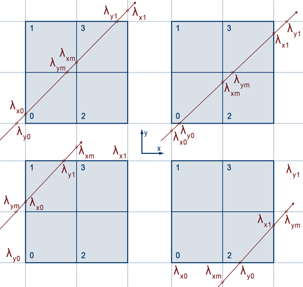
In Figure4, The triangle and square in each column are in identical positions. The one on top is visualizing the projections onto the separating axes defined by the vector orthogonal to the triangle's edges, while the bottom is visualizing the projections onto the ones defined by vectors orthogonal to the square's edges. The axes are represented by bold lines. Gaps are highlighted in green, and overlaps are highlighted in red.
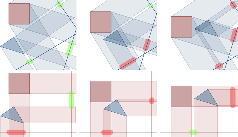
To better visualize this, take a look at this interactive demo (Flash is required) by dragging the rectangle (which represents the AABB) around. It's a simplified case where two edges of the triangle happen to be parallel to the sides of the rectangle, but the idea of using a separating axis perpendicular to the polygon's edge is well demonstrated.
For a 3D AABB, it can be simplified into the 2D case by projecting the AABB and triangle down each of the three $x$, $y$, and $z$ axis. In other words, we can turn the 3D space into three 2D spaces by projecting down the $x$ axis onto the $YZ$ plane, $y$ axis onto the $XZ$ plane, and $z$ axis onto the $XY$ plane. The same overlap tests as shown in Figure4 can then be executed for each projection. This sums up to 15 tests: 5 tests on the separating axes, multiplied by 3 projections. We return no overlap if any one of these tests find a gap.
There is a problem with this simplification however, as the case demonstrated in Figure5 shows.
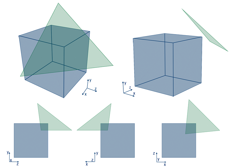
This is because there's a separating axis that exists in 3D, but not in 2D: the triangle's normal vector. Another test along the separating axis defined by the triangle's normal is needed. After all 16 tests have completed without finding a gap, we can be sure that the triangle isn't intersecting / overlapping with the AABB.
As mentioned above, the 15 tests comes from the 3 different 2D projections. The 5 tests executed for each projection are essentially the same, so we will only go over one of the axes; the $x$ axis projection onto the $YZ$ plane.
In Figure6, the projection onto the $YZ$ plane is visualized. The five vectors that are orthogonal to each of the two polygons' edges are drawn on the projection. They define the direction vectors of the separating axes to test, and we will refer to them as the edge normals.
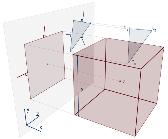
For simplicity, the first thing we do is to translate the AABB and triangle such that the AABB's center $c$ is at the origin $[0,0,0]$. This can be easily calculated by subtracting the triangle vertices $\vec t_0,\vec t_1,\vec t_2$ and $c$ itself by $c$. We will assume that $c$ is at the origin from this point forth.
Finding these edge normals are quite easy if we notice their properties. First, notice that they are all orthogonal to the $x$ axis, as they exist on the $YZ$ plane. In addition, they must be orthogonal to the edges of the polygon, as that is the definition of a normal vector. Therefore, the projected edge normals can be easily calculated as a cross product of the $x$ unit vector, and the polygon's edge.
We will first look at the AABB's edge normals. A cross product calculation is not necessary to find them, as we know the AABB is axis aligned. Therefore, the normals to these edges must also be axis aligned. In this case, they are simply the unit vectors $\hat e_y = [0, 1, 0]$ and $\hat e_z = [0, 0, 1]$. We will also define $\hat e_x = [1, 0, 0]$ for completeness.
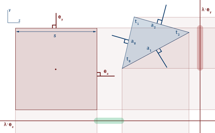
Projecting onto $\hat e_y$ and $\hat e_z$ and then checking for overlaps is also easy. An overlap on the projection onto $\hat e_y$ can be found if the range $[min(t_{0y}, t_{1y}, t_{2y}), max(t_{0y}, t_{1y}, t_{2y})]$ overlaps the range $[-s/2, +s/2]$. The same can be done for the projection onto $\hat e_z$, by using the $z$ components of the vectors. Note that this is equivalent of finding the overlap between the projected AABB, and the minimum AABB around the projected triangle.
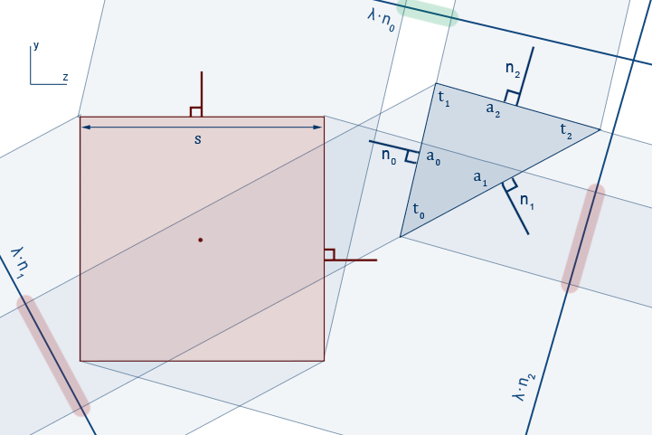
Unlike the edges of the AABB, the triangle's edges can be arbitrary. Therefore, we will need to find its edge normals using the cross product.
As shown in Figure8, Let $\vec t_0,\vec t_1,\vec t_2$ be the triangle's vertices, $\vec a_0,\vec a_1,\vec a_2$ be the triangle's edges, and $\vec n_0,\vec n_1, \vec n_2$ be the respective edge normals. We can find $\vec a_i$ as follows:
$$\begin{align*} \vec a_0 = \vec t_1 - \vec t_0\\ \vec a_1 = \vec t_2 - \vec t_0\\ \vec a_2 = \vec t_2 - \vec t_1 \end{align*}$$
We then find $\vec n_i$ using the cross product:
$$\begin{align*} \vec n_0 = \hat e_x \times \vec a_0 = [0, -a_{0z}, a_{0y}] = [0, t_{0z}-t_{1z}, t_{1y}-t_{0y}]\\ \vec n_1 = \hat e_x \times \vec a_1 = [0, -a_{1z}, a_{1y}] = [0, t_{0z}-t_{2z}, t_{2y}-t_{0y}]\\ \vec n_2 = \hat e_x \times \vec a_2 = [0, -a_{2z}, a_{2y}] = [0, t_{1z}-t_{2z}, t_{2y}-t_{1y}]\\ \end{align*}$$
After finding the three $\vec n_i$'s, we project the triangle vertices onto each one. We will project onto $\vec n_0$ as an example, since the other two use similar calculations.
$$\begin{align*} proj_{\vec n_0}\vec t_0 &= \vec n_0\cdot\vec t_0 = [0, -a_{0z}, a_{0y}]\cdot[t_{0x}, t_{0y}, t_{0z}] = t_{0z}t_{1y}-t_{0y}t_{1z}\\ proj_{\vec n_0}\vec t_1 &= \vec n_0\cdot\vec t_1 = [0, -a_{0z}, a_{0y}]\cdot[t_{1x}, t_{1y}, t_{1z}] = t_{0z}t_{1y}-t_{0y}t_{1z} = proj_{n_0}\vec t_0\\ proj_{\vec n_0}\vec t_2 &= \vec n_0\cdot\vec t_2 = [0, -a_{0z}, a_{0y}]\cdot[t_{2x}, t_{2y}, t_{2z}] = t_{2y}(t_{0z}-t_{1z})+t_{2z}(t_{1y}-t_{0y})\\ \end{align*}$$
Note that $proj_{\vec n_0}\vec t_0=proj_{\vec n_0}\vec t_1$, which makes sense since the projections of $\vec t_0$ and $\vec t_1$ onto $\vec n_0$ results in a single point. As a result, we now know that the triangle occupies a range of $[min(proj_{\vec n_0}\vec t_0, proj_{\vec n_0}\vec t_2),max(proj_{\vec n_0}\vec t_0, proj_{\vec n_0}\vec t_2)]$ within the projection onto $\vec n_0$.
Since the AABB is a cube, its size across all three axis is identical. Given that its center is at the origin, we can find the "radius" $r$ it occupies on the projection onto $\vec n_0$. Let $s_h = s/2$ denote the half-sze of the AABB, and $|\cdot|$ represent absolute value. Then,
$$\begin{align*} r &= \vec s_h \cdot |\vec n_0|\\ &= s_h|n_{0x}| + s_h|n_{0y}| + s_h|n_{0z}|\\ &= s_h|n_{0y}| + s_h|n_{0z}\\ \end{align*}$$
Where $s_h|n_{0x}|$ is eliminated since $n_{0x} = 0$
The absolute value has the effect of mirroring the negative components of $\vec n_0$ such that the AABB's diagonal half vector $[s_h, s_h, s_h]$ will be properly projected onto it with the right orientation. We can do this since the AABB is fully symmetrical across its center $\vec c = [0,0,0]$. Therefore, the AABB occupies a range of $[-r, r]$ within the projection onto $\vec n_0$.
Finally, checking for an overlap on the projection boils down to checking if the ranges $[min(proj_{\vec n_0}\vec t_0, proj_{\vec n_0}\vec t_2),max(proj_{\vec n_0}\vec t_0, proj_{\vec n_0}\vec t_2)]$ and $[-r, r]$ overlap. We then repeat the process, with slightly different but similar equations as shown above, for $\vec n_1$, and $\vec n_2$.
The five axes tests are then repeated for the other two projections, namely the projections onto the $XY$, and $XZ$ planes. If during the process, any of these tests identifies a gap within the projection, then we immediately know that the triangle and AABB do not overlap.
If we do not identify a gap within any of these 15 tests, we execute the final 16th test on the separating axes defined by the triangle's normal. If even this test does not find a gap, then we are certain that the triangle is overlapping the AABB.
There is a small optimization that can be made to the series of 15 tests. If we observe the total of 6 axes tests done using the unit vectors $\hat e_x, \;\hat e_y, \;\hat e_z$, we see that they are being done twice:
Therefore, we can move these tests into its own category, executing one test for each of the $\hat e_i$'s. This gives us a total test count of 13 instead of 16.
Using the triangle-AABB intersection algorithm, we will be able to identify the triangles in a node that is intersecting with its children. This is done during the subdivide phase of the 3-greedy algorithm to create $T^{complete}_3$. As we're subdividing at each level, the triangles within the current node are partitioned off into its 8 children. This prepares $T^{complete}_3$ for the pruning phase, where the cost function uses the number of triangle contained within the leaves to compute $C_o(T)$.
Now that we've constructed the octree, we have to be able to cast rays within it to find triangle-ray intersections. As it turns out, the recursive and cubic nature of octree nodes makes this process fast and elegant.
As mentioned in the introduction, ray-tracing with an octree involves sending a ray into the octree structure, and finding the sequence of leaves that the ray will hit, sorted in order of hit distance. For each intersected leaf, we query its list of triangle for intersections. If one exists, we check that the hit point is within the confines of the leaf. If it is, we return the ray-triangle intersection information. Otherwise, we continue to the next leaf within the traversal, and repeat the process.
Although it is possible to traverse the leaves in arbitrary order, it is sub-optimal. Any $\lambda$ values found can only be seen as candidates, since there might exist another leaf containing a triangle that results in a smaller $\lambda$ value. Searching through the leaves in order of hit ($\lambda$) distance will give us the assurance that the first valid ray-triangle intersection is the closest one.
Due to the recursive structure of the octree, identifying the intersected leaves in order can be done fast, and elegantly. The algorithm that was used in this implementation is presented in An Efficient Parametric Algorithm for Octree Traversal. An explination of the paper, with more focus on the 3D generalization, can be found here. As usual, we will simplify the 3D problem down to 2D for simplicity, and then generalize to 3D.
In the 2D case, our octree squashes down to a quadtree, where each node has only 4 children. We will also assume, for now, that the components for the direction vector of the ray are all positive. In the end, the concept will be extended to 3D, using rays with arbitrary direction vectors.
When a ray intersects with a node (an AABB), we know that it must enter the AABB at some $\lambda$, and exit at some $\lambda$. We also know that if a node is being intersected by a ray, some of its children must also be intersected by it. The algorithm then must recurse on the intersected children, repeating the process we've just described. The questions are:
We'll start by defining our terms.
| Term | Definition |
|---|---|
| $r(\lambda) = \vec p + \lambda \vec d$ | The ray, defined by its origin $\vec p$ and direction vector $\vec d$. A point on the line is given by different values of $\lambda$ |
| $\phi$ | Represents an arbitrary axis. Can be $x$ or $y$ in the 2D case. |
| $\phi _r(\lambda) = p_{\phi } + \lambda d_{\phi }$ | Parametric equation for the $\phi $ component of ray $r$. For example, the $x$ parametric equation is $x_r(\lambda) = p_x + \lambda d_x$ |
| $t = (x_0, y_0, x_1, y_1)$ | A node within the quadtree. It is defined by its min and max boundary values such that a point $\vec p$ within the node must satisfy $x_0 \leq p_x \lt x_1 \land y_0 \leq p_y \lt y_1$ |
| $\lambda_{\phi i}(t,r)$ | The $\lambda$ value for ray $r$ at its intersection point with the boundary $\phi_i$ of node $t$. For example, $\lambda_{x0}(t, r)$ is the $\lambda$ value for ray $r$ at its intersection with the boundary $x_0$ of node $t$. It is abbreviated as $\lambda_{\phi i}$ ($\lambda_{x0}$, for example) when the context for $(t,r)$ is given. |
Before we continue, is good to keep in mind that the algorithm described is recursive. We will use the root node to simplify explanations. But since the quadtree structure is recursive, the root node can - in reality - be any node $t$ within the quadtree.
Let us first consider the conditions in which a line is considered to be overlapping a node defined by its min and max vertices. A ray $r$ will intersect node $t$ if and only if there exists $\lambda \in \mathbb{R}$ such that
$$x_0(t) \leq x_r(\lambda) \lt x_1(t) \land y_0(t) \leq y_r(\lambda) \lt y_1(t)$$
Where $\phi _i(t)$ returns the specified boundary value of node $t$. Looking at this from a different perspective, we can think of the range of $\lambda$'s that satisfies the above to be within $\lambda_0 \leq \lambda \lt \lambda_1$. This implies that $\lambda_0$ and $\lambda_1$ must be the inputs to $r$ such that $r(\lambda_0)$ is the point of entry, and $r(\lambda_1)$ is the point of exit.
Given the boundaries of the node's AABB, we can check to see if $r$ intersects $t$ by solving for $\lambda_0$ and $\lambda_1$ using $r$'s parametric equation.

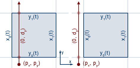
Finding $\lambda_0$ and $\lambda_1$ involves solving for $\lambda_{\phi i}$'s as shown in Figure9:
$$\begin{align*} x_i(t) &= x_r(\lambda_{xi}) \implies & x_i(t) &= p_x+\lambda_{xi}d_x \implies & \lambda_{xi} &= \frac{x_i(t)-p_x}{d_x}\\ y_i(t) &= y_r(\lambda_{yi}) \implies & y_i(t) &= p_y+\lambda_{yi}d_y \implies & \lambda_{yi} &= \frac{y_i(t)-p_y}{d_y}\\ \end{align*}$$
Notice that for $\lambda_{x0}$ and $\lambda_{y0}$, the entry $\lambda_0 = max(\lambda_{x0},\lambda_{y0})$. The same foes for $\lambda_{x1}$ and $\lambda_{y1}$, where the exit $\lambda_1 = min(\lambda_{x1}, \lambda_{y1})$.
If the inequality $\lambda_0 \leq \lambda_1$ holds, and $\lambda_1 \gt 0$, then ray $r$ is intersecting node $t$. We check that $\lambda_1$ is positive to ignore AABB intersections that are "behind" the ray.
Looking at the equations for $\lambda_{\phi i}$, we see that their values can be $\infty$ depending on whether $d_x$ or $d_y$ is 0. Whether it is $+\infty$ or $-\infty$ depends on the sign of $\phi _i(t)-p_{\phi }$
We observe the following from Figure10:
The same will be observed if we make the $x$ component of $d$ zero.
Now that we know that $r$ is intersecting with the root node, we have to determine the series of children nodes that will be intersected. The possible entry nodes, assuming that the ray's direction components are all positive, are children 0, 1, and 2. We can use this, along with $r$'s midplane intersection lambdas: $\lambda_{xm},\;\lambda_{ym}$ and entry plane intersection lambdas: $\lambda_{x0},\;\lambda_{y0}$ to figure out which of the three indices is the actual entry node.
Calculating $\lambda_{\phi m}$ is easy. We take the average of the entry and exit $\lambda$'s for each axis:
$$\lambda_{\phi m} = \frac{\lambda_{\phi 0}+\lambda_{\phi 1}}{2}$$
Looking at Figure11, we see that when $\lambda_{x0}\gt\lambda_{y0}$ (the first column), the possible children we can enter are 0 and 1. However, when $\lambda_{x0}\lt\lambda_{y0}$ (2nd column), the possible children are 0 and 2.
First, note that $\lambda_0=\lambda_{x0}$ in the first column, while $\lambda_0=\lambda_{y0}$ in the second. We see that the axis corresponding to the lambda returned by $max(\lambda_{x0}, \lambda_{y0})$ also represents the normal to the line in which the ray intersects to enter the node. In the 2D case, we will call this the entry line, which is simply either the $X$ line, or the $Y$ line. In the 3D case, they would be the entry planes: $XY$, $YZ$, or $XZ$ planes.
| Maximum | Entry line |
|---|---|
| $\lambda_{x0}$ | $Y$ |
| $\lambda_{y0}$ | $X$ |
When $\lambda_{y0}\lt\lambda_0$ ($Y$ is entry line since $\lambda_0 = \lambda_{x0}$), we see whether we're entering node 0 or 1 by checking if $\lambda_{ym}\lt\lambda_0$. If it is, 1 is the entry node, or 0 otherwise. Likewise when $\lambda_{x0}\lt\lambda_0$ ($X$ is entry line since $\lambda_0 = \lambda_{y0}$), we check if $\lambda_{xm}\lt\lambda_0$. If it is, 2 is the entry node, or 0 otherwise.
If we're observant, a slight convenience will pop up. With the order that we're indexing the children nodes, and the knowledge of the entry line, we can use bit operations to determine the entry node. This changes the code from:
entryNode = 0;
if (lambda_x0 < lambda_0 && lambda_xm < lambda_0) entryNode = 2;
if (lambda_y0 < lambda_0 && lambda_ym < lambda_0) entryNode = 1;
To:
entryNode = 0;
// | is the inclusive or bit operator.
if (entryLine = X && lambda_ym < lambda_0) entryNode |= 2;
if (entryLine = Y && lambda_xm < lambda_0) entryNode |= 1;
In the 2D case, using bit operations seems pointless. But this is because there is only two axes. In 3D, using bit operations will significantly reduce the number of conditionals
Now that the entry node is identified, we need to find the next child node(s) after we've finished processing the entry node.
Going back to Figure11 we see that the next child node we traverse into depends on
Based upon the above, we can deduce the next children, and the next children after that, until we've exited the current node.
The current child node we are in can be tracked with an integer indicating its index. Knowing this, we can calculate its exit line quite easily. Looking at Figure11, we construct the following table of nodes and their possible exit $\lambda$'s:
| Current child node | Exit lambda |
|---|---|
| 0 | $min(\lambda_{xm},\lambda_{ym})$ |
| 1 | $min(\lambda_{xm},\lambda_{y1})$ |
| 2 | $min(\lambda_{x1},\lambda_{ym})$ |
| 3 | $min(\lambda_{x1},\lambda_{y1})$ |
Depending on which $\lambda_{\phi i}$ was found as the minimum, it defines the exit line that the ray will cross over.
| Minimum | Exit line |
|---|---|
| $\lambda_{xi}$ | $Y$ |
| $\lambda_{yi}$ | $X$ |
Furthermore, depending on the current child node, and which exit line the ray crosses over, we find the next child node in the sequence.
| Current child node | Exit Line $X$ | Exit Line $Y$ |
|---|---|---|
| 0 | 1 | 2 |
| 1 | EXIT | 3 |
| 2 | 3 | EXIT |
| 3 | EXIT | EXIT |
For example, if current node is 0, and $\lambda_{xm} = min(\lambda_{xm},\lambda_{ym}) \implies$ exit line $Y$, then the next node in the traversal is child 2. But if $\lambda_{ym} = min(\lambda_{xm},\lambda_{ym}) \implies$ exit line $X$, then the next node is child 1.
Programatically, this is best though of as a do-while loop:
do {
    Find curNode's exit lambdas according to above tables.
    Find lambda_1m = min(exit lambdas).
    Find the nextNode respective to lambda_1m.
    Process curNode via recursive call.
    Set curNode = nextNode.
} while (curNode != EXIT)
To account for negative components in $\vec d$, we employ a trick on how we index the child nodes. The idea is that the ray doesn't need to know about the triangles contained within a node until it has reached a leaf. Therefore, we can mirror the the quadtree and the ray such that the components within $\vec d$ become all positive.

To mirror ray $r$ such that $\vec d$ is all positive, we first create a copy of it. In the copied ray, we mirror its origin $\vec p$ across the AABB's center $\vec c$ in the directions of the axis that are negative within $\vec d$. Likewise, we flip the sign on the negative components of $\vec d$.
To mirror the node, we employ a different indexing scheme to the child nodes, such that what use to be, say child 0, becomes child 1, and what use to be child 1, becomes child 0. This new scheme of indexing, along with the copied ray, effectively mirrors the quadtree and ray in the direction of the negative $\vec d$ components.
To tell the algorithm to use the new indexing scheme, we pass the modified child index in place of the usual one within the recursive call. This modified index is the usual index modified with another number that "flips" it. For example, consider the top row within Figure12. If we only flip the ray but not the node, we see that the ray will first cross 0. But since we're also flipping the node by changing its indexing scheme, what use to be 0 now becomes 1, and what use to be 1 becomes 0. Therefore, in the recursive step, we pass in child 1 in place of child 0. We can again, do this modification with bit operations. First we make a table of the changes we observe to the entry nodes as seen from Figure12:
| Entry line | $+x,\;+y$ | $+x,\;-y$ | $-x,\;-y$ |
|---|---|---|---|
| $X$ | 0, 2 | 1, 3 | 3, 1 |
| $Y$ | 0, 1 | 1, 0 | 3, 2 |
The possible next child nodes, in addition to the current child node (CCN), will also change. As seen in Figure12:
| $+x,\;+y$ | $+x,\;-y$ | $-x,\;-y$ | ||||||
|---|---|---|---|---|---|---|---|---|
| CCN | $X$ | $Y$ | CCN | $X$ | $Y$ | CCN | $X$ | $Y$ |
| 0 | 1 | 2 | 1 | 0 | 3 | 3 | 2 | 1 |
| 1 | 4 | 3 | 0 | 4 | 2 | 2 | 4 | 0 |
| 2 | 3 | 4 | 3 | 2 | 4 | 1 | 0 | 4 |
| 3 | 4 | 4 | 2 | 4 | 4 | 0 | 4 | 4 |
The pattern is that there seems to be a bit correspondence with each axis. $x$ seems to correspond to 2, which is 10 in binary, and $y$ seems to correspond to 1, which is 1 in binary. To see why, pick a column within either Table7 or Table8, and calculate the flip integer like so:
flip = 0;
if (x < 0) flip |= 2;
if (y < 0) flip |= 1;
Then, take the number(s) under the $+x,\;+y$ column and XOR it with flip. The result is the same number as the ones under the column you've picked, with the exception of 4, since its binary representation '100' is three bits long. 4 ^ flip will only generate a number greater than or equal to 4.
Therefore, mirroring the current node is as simple as finding which components of the ray's direction vector $\vec d$ is negative, composing the flip integer, and applying a few XORs. This procedure need only be applied during the recursive step when we're specifying which node to recurse on, effectively mirroring the tree. All other procedures remain identical:
do {
    Find curNode's exit lambdas according to above tables.
    Find lambda_1m = min(exit lambdas).
    Find the nextNode respective to lambda_1m.
    Process (curNode ^ flip) via recursive call.
    Set curNode = nextNode.
} while (curNode < 4)
The 3D case involves more cases to consider, but the concept is identical to the 2D case.
On top of $\lambda_{xi}$ and $\lambda_{yi}$ we now have $\lambda_{zi}$ as well. Finding $\lambda_0$ and $\lambda_1$ now involves finding $max(\lambda_{x0}, \lambda_{y0}, \lambda_{z0})$ and $min(\lambda_{x1}, \lambda_{y1}, \lambda_{z1})$ respectively. Checking $\lambda_0\lt\lambda_1 \land lambda_1 \gt 0$ as usual will determine if there is an intersection.
Nothing changes for the parallel cases. The final $\lambda_0\lt\lambda_1$ checks for this.
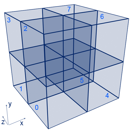
This is where the major difference between the 2D and 3D cases start. First, an octree node's children will have to be indexed differently, as there is now 8 children. Figure1 shows the indexing order we'll be using. This means that with a ray $r$ containing a direction vector $\vec d$ with positive components, the possible entry child nodes are everything except for index 7.
Also the concept of the entry line doesn't exit anymore. in 3D, we look at the three possible entry and exit planes: $YZ,\;XZ,$ and $XY$. Identifying the entry plane however, uses the same approach of finding the axes corresponding to the maximum entry lambda, then finding the plane that is orthogonal to it.
Using the bit operations approach to identify the specific entry child node:
entryNode = 0;
if (entryPlane == YZ){
    // => lambda_0 = lambda_x0
    if (lambda_ym < lambda_0) entryNode |= 2;
    if (lambda_zm < lambda_0) entryNode |= 1;
}
else if (entryPlane == XZ){
    // => lambda_0 = lambda_y0
    if (lambda_xm < lambda_0) entryNode |= 4;
    if (lambda_zm < lambda_0) entryNode |= 1;
}
else{
    // (entryPlane == XY) => lambda_0 = lambda_z0
    if (lambda_xm < lambda_0) entryNode |= 4;
    if (lambda_ym < lambda_0) entryNode |= 2;
}
Which is the logical equivalent of
entryNode = 0;
if (entryPlane != YZ && lambda_mx < lambda_0) entryNode |= 4;
if (entryPlane != XZ && lambda_my < lambda_0) entryNode |= 2;
if (entryPlane != XY && lambda_mz < lambda_0) entryNode |= 1;
As mentioned previously, the bit operations reduces the number of conditionals.
The 3D case is just a expansion of the 2D case by adding more rows to our table. To figure out what goes within these new rows, the best way is to diagram them out, similar to what was done in Figure12. Without adding additional images, here are the tables for the 3D case:
We construct the following table of nodes and their possible exit λ's:
| Current child node | Exit lambda |
|---|---|
| 0 | $min(\lambda_{xm},\lambda_{ym},\lambda_{zm})$ |
| 1 | $min(\lambda_{xm},\lambda_{ym},\lambda_{z1})$ |
| 2 | $min(\lambda_{xm},\lambda_{y1},\lambda_{zm})$ |
| 3 | $min(\lambda_{xm},\lambda_{y1},\lambda_{z1})$ |
| 4 | $min(\lambda_{x1},\lambda_{ym},\lambda_{zm})$ |
| 5 | $min(\lambda_{x1},\lambda_{ym},\lambda_{z1})$ |
| 6 | $min(\lambda_{x1},\lambda_{y1},\lambda_{zm})$ |
| 7 | $min(\lambda_{x1},\lambda_{y1},\lambda_{z1})$ |
Depending on which $\lambda_{\phi i}$ was found as the minimum, it defines the exit plane that the ray will cross over.
| Minimum | Exit plane |
|---|---|
| $\lambda_{xi}$ | $YZ$ |
| $\lambda_{yi}$ | $XZ$ |
| $\lambda_{zi}$ | $XY$ |
Furthermore, depending on the current child node, and which exit plane the ray crosses over, we find the next child node in the sequence.
| Current child node | Exit Plane $YZ$ | Exit Plane $XZ$ | Exit Plane $XY$ |
|---|---|---|---|
| 0 | 4 | 2 | 1 |
| 1 | 5 | 3 | EXIT |
| 2 | 6 | EXIT | 3 |
| 3 | 7 | EXIT | EXIT |
| 4 | EXIT | 6 | 5 |
| 5 | EXIT | 7 | EXIT |
| 6 | EXIT | EXIT | 7 |
| 7 | EXIT | EXIT | EXIT |
Much like the 2D case, there is an axis-bit correspondence in 3D. $x$ corresponds with 4, or 100 in binary, $y$ corresponds with 2, or 10 in binary, and $z$ corresponds with 1, or 1 in binary.
Constructing the flip integer, and applying it to child node indices works the same way as in 2D. Only difference is we also have to check if the $z$ component from the direction vector $\vec d$ is negative.
To tie everything together, the following pseudo-code explains the procedure for recursive, top-down ray casting. Here's a list of the functions we'll be using as an outline:
cast_ray(OctNode root, Ray R)
    // Return the ray-triangle intersection information, such as the lambda,
    // normal, and texture coordinates.
compute_lambdas(OctNode t, ray R, double lambda_0s[3], double lambda_1s[3])
    // Return void, but sets the respective lambdas for ray R given the
    // octree node.
process_subtree(double lambda_0s[3], double lambda_1s[3], int flip,
                Ray R, OctNode t)
    // Return the ray-triangle intersection information, if one was found.
next_node(double lambda_1s[3], int possibleNextNodes[3])
    // Return the respective next node, or 8 for exit, depending on which exit
    // lambda is the minimum. Passing in the possible next nodes reduces the
    // number of conditionals.
tri_intersect(OctNode t, Ray R)
    // Return the intersection info if R intersects some triangle within the
    // bounds of the AABB defined by t.
We will write the pseudo-code for cast_ray and process_subtree only, since the other ones are straight forward:
IntersectInfo cast_ray(OctNode root, Ray R){
    int flip = 0;
    Ray copyR = R.getCopy();
    // Calculate the flip integer used to "mirror" the scene.
    // Don't forget to mirror the ray's origin across the nodes center.
    if(copyR.d.x < 0) {
        copyR.o.x = 2*root.center.x - R.o.x;
        copyR.d.x = -copyR.d.x;
        flip |= 4;
    }
    if(copyR.d.y < 0) {
        copyR.o.y = 2*root.center.y - R.o.y;
        copyR.d.y = -copyR.d.y;
        flip |= 2;
    }
    if(copyR.d.z < 0) {
        copyR.o.z = 2*root.center.z - R.o.z;
        copyR.d.z = -copyR.d.z;
        flip |= 1;
    }

    double lambda_0s[3], lambda_1s[3];
    // Find the root node's entry and exit lambdas.
    compute_lambdas(root, copyR, lambda_0s, lambda_1s);
    double lambda_0 = max(lambda_0s);
    double lambda_1 = min(lambda_1s);

    // Check if the intersection is valid.
    if (lambda_1 <= 0 || tmin > tmax) return NULL;

    // At this point, copyR is not needed anymore. The lambda value are enough
    // to deduce any future AABB-ray intersections.
    // However, R is needed for finding ray-triangle intersections.
    return process_subtree(lambda_0s, lambda_1s, flip, R, root);
}

IntersectInfo process_subtree(double l_0s[3],double l_1s[3],
int flip, Ray R, OctNode t){
    int curNode;
    // Ignore this node if it is behind the ray origin.
    if (has_negative_components(l_1s)) return;

    // Find entry and exit lambdas, in addition to the entry plane.
    double l_0 = max(l_0s);
    double l_1 = min(l_1s);
    // find_entry_plane() will return the axis that is normal to the entry plane
    int entryPlane = find_entry_plane(l_0s); // 0 for X, 1 for Y, 2 for Z.

    if (t.isLeaf()) return tri_intersect(t, R);

    // Calculate the midplane lambdas.
    double l_ms[3];
    l_ms[0] = l_0s[0] + l_1s[0] / 2;
    l_ms[1] = l_0s[1] + l_1s[1] / 2;
    l_ms[2] = l_0s[2] + l_1s[2] / 2;

    // Find first node intersected out of the 8.
    curNode = 0;
    if (entryPlane != 0 && l_ms[0] < l_0) curNode |= 4;
    if (entryPlane != 1 && l_ms[1] < l_0) curNode |= 2;
    if (entryPlane != 2 && l_ms[2] < l_0) curNode |= 1;

    // The entry and exit lambdas for child nodes.
    double cl_0s[3], cl_1s[3];
    int nextNodes[3];
    IntersectInfo intersect;
    do {
        // For the current node, identify its entry and exit lambdas.
        // Set the possibilities for its next nodes.
        if (curNode == 0){
            cl_0s = {l_0s[0], l_0s[1], l_0s[2]}
            cl_1s = {l_ms[0], l_ms[1], l_ms[2]}
            nextNodes = {4, 2, 1};
        }
        else if (curNode == 1){
            cl_0s = {l_0s[0], l_0s[1], l_ms[2]}
            cl_1s = {l_ms[0], l_ms[1], l_1s[2]}
            nextNodes = {5, 3, 8};
        }
        else if (curNode == 2){
            cl_0s = {l_0s[0], l_ms[1], l_0s[2]}
            cl_1s = {l_ms[0], l_1s[1], l_ms[2]}
            nextNodes = {6, 8, 3};
        }
        else if (curNode == 3){
            cl_0s = {l_0s[0], l_ms[1], l_ms[2]}
            cl_1s = {l_ms[0], l_1s[1], l_1s[2]}
            nextNodes = {7, 8, 8};
        }
        else if (curNode == 4){
            cl_0s = {l_ms[0], l_0s[1], l_0s[2]}
            cl_1s = {l_1s[0], l_ms[1], l_ms[2]}
            nextNodes = {8, 6, 5};
        }
        else if (curNode == 5){
            cl_0s = {l_ms[0], l_0s[1], l_ms[2]}
            cl_1s = {l_1s[0], l_ms[1], l_1s[2]}
            nextNodes = {8, 7, 8};
        }
        else if (curNode == 6){
            cl_0s = {l_ms[0], l_ms[1], l_0s[2]}
            cl_1s = {l_1s[0], l_1s[1], l_ms[2]}
            nextNodes = {8, 8, 7};
        }
        else if (curNode == 7){
            cl_0s = {l_ms[0], l_ms[1], l_ms[2]}
            cl_1s = {l_1s[0], l_1s[1], l_1s[2]}
            nextNodes = {8, 8, 8};
        }
        // Recursively call process_subtree.
        // If an intersection is found in recursive call, return it.
        // Otherwise, find the next node in the traversal and continue
        // searching.
        // Note that we "mirror" the tree using the flip constant.
        intersect = process_subtree(cl_0s, cl_1s, flip, R,
                        node.getChild(curNode^flip));
        if (intersect) return intersect;
        // Find the next nodes
        curNode = next_node(cl_1s, nextNodes);
    } while (curNode < 8);
    return NULL; // Exited current node without finding any intersections.
}
The octree construction and ray-casting algorithms were coded in C++. The below performance tests were performed on a machine with an Intel® Core™ i7-2600K processor, and 16GB of RAM. Although the processor supports 8 threads, the code was ran single-threaded for consistency.
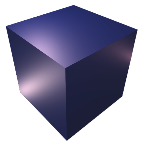
The test scenes were all a simple cube, with varying tessellation levels to achieve the desired triangle count. The scenes varied from 180 triangles, up to 1048576 triangles. The camera orientation, position, and field of view were kept consistent throughout all scenes to ensure that the cube occupied the same number of pixels. The output image size was 1024x1024, with no anti-aliasing.
The data gathering method involves coding a timer within the ray-tracer, starting and ending at desired points within the program. We then run the ray-tracer on the various cube scenes. Scenes that have low triangle counts are fast to render, generating noisy results. Therefore, we run these scenes 10 to 20 times, averaging the results to produce a more accurate number.
Running the ray-tracer multiple times for scenes that took more than 1 hour were not necessary, as any noise would have had a negligible effect on the result. Therefore, running the naive method on scenes with more than 100,000 triangles were only done once.
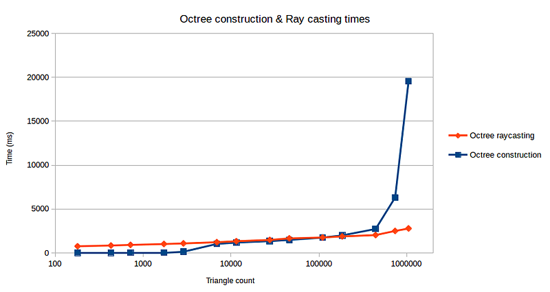
Although the octree construction times scale linearly with the number of triangles, the ray-casting times scales logarithmically. This is a desirable trait to have, since triangle count in many 3D scenes can get quite large.
It is unclear why the construction times suddenly spiked between triangle counts 1000 and 10000. The scenes in this range were ran multiple times, yielding the same results.
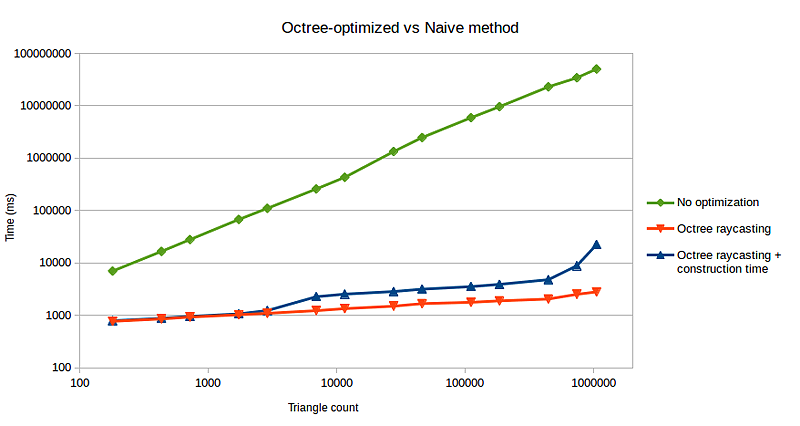
As expected, the naive method takes exponentially longer compared to the octree method as triangle counts increase.
In this report, we constructed the octree by using a cost function that is proven to be optimal, in addition with a fast triangle-AABB intersection algorithm to partition the triangles into the octree leaves. Due to the octree's recursive and cubic structure, executing the ray-casting procedure is fast and relatively simple. We used an algorithm that takes an top-down approach to traversing the octree, which reduced the number of operations required by ignoring leaves that are not within the ray's path. This sums up to a fast algorithm with run-times that is logarithmically related to the scene's triangle count.
Although the code can be considered complete, aspects of it can still be optimized. Coherence between different functions in the octree library can be improved, and a few conditional statements can be optimized further. However, improvements and optimizations should be made while keeping in mind the educational purpose of this ray-tracer, as some improvements may need to be sacrificed for the sake of code readability.
Throughout the project course, a few feature unrelated to the octree was implemented. Here's a list of the features, and their respective documents for reference.
